
Use dimensional analysis and educated guessing to simplify experimentation and simulation, gain physical insight from empirical relationships, and extrapolate data.
Dimensional analysis is a powerful tool that can be used to obtain insight into complex problems at very little cost. In engineering curricula, it is primarily used to introduce the concept of similarity in the context of scale models. Students also learn how to apply dimensional analysis to academic problems, such as determining the period of oscillation of a pendulum without solving a differential equation, estimating the walking speed of dinosaurs starting from fossil footprints (1), or explaining the color of the sky without referring to Maxwell’s equations (2).
However, dimensional analysis is largely overlooked as an analytical tool for engineering applications. When textbook methods of dimensional analysis are applied to practical engineering problems, they generally yield obscure relationships that are not very informative. Indeed, successful application of dimensional analysis relies on some form of educated guessing. This step is often implicit in the classroom coverage of the problems, which leaves students and practitioners alike unfamiliar with this tactic. This article discusses the many insights dimensional analysis and educated guessing give into the complex question of liquid holdup in trickle-bed reactors.
The basics of dimensional analysis

The principle of dimensional analysis is that any quantitative result should hold true independent of units. The outcome of any experiment or calculation may be formalized as a functional dependence between an unknown output variable, v0, and a series of input variables, v1, v2 …, that characterize the system:
The form of the function f is what any study aims to uncover by either experimental or theoretical means. For example, in the context of heat exchange, the heat flux (v0) between an object and a surrounding fluid depends on the temperature difference between the object and the fluid (v1), the heat conductivity of the fluid (v2), the width (v3), length (v4),and height (v5) of the object, the fluid’s viscosity (v6), and density (v7), and more. If the temperatures were expressed in Fahrenheit rather than Celsius, the numerical values of v1 and v2 would be different but Eq. 1 should still be satisfied. The same holds true if lengths are expressed in meters rather than inches, or times in minutes rather than seconds.
The units of the dimensional variables v0, v1… are rooted in the laws of physics. For example, stating that the heat conductivity has the dimensions W-m–2-K–1 implies that heat fluxes (W-m–2) are proportional to temperature differences (K). To make a system compatible with the basic laws of physics, relationships such as those in Eq. 1 must be invariant with respect to arbitrary changes of units. The constraints that this invariance puts on the possible forms of f are very informative to an engineer.

The central theorem of dimensional analysis is the Buckingham Π theorem (3, 4), which states that the only way to make Eq. 1 invariant with respect to the units is to write it in terms of dimensionless variables:

where each variable Πi is a product:
and the exponents ai, bi, ci … are chosen to make Πi dimensionless.
Buckingham’s theorem is insightful, as there are fewer dimensionless variables Πi than the corresponding dimensional variables vi. The number of independent dimensionless variables is equal to the number of dimensional variables (input and output) minus the number of independent units in the problem. Applying this procedure to the variables relevant to heat transfer yields the classical dimensionless groups known as the Nusselt, Reynolds, and Prandtl numbers (5), which are commonly used for the design of scale models.
Any dependence incompatible with Eq. 2 would not be invariant upon a change of units. Therefore, it is not merely a convenience to express a problem in terms of dimensionless variables — it is a logical necessity.
The sidebar at the end of this article explains an alternative approach to dimensional analysis.
Illustration with trickle-bed reactors
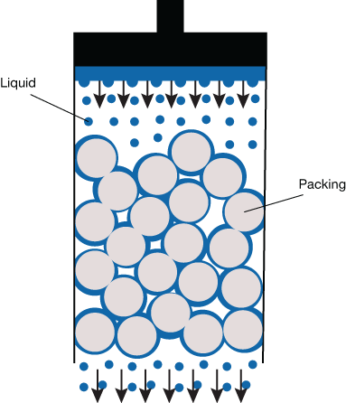
▲Figure 1. In a trickle-bed reactor, a liquid (blue) is poured over packing with a complex geometry (gray) to maximize the contact between the liquid and the gas. One value of interest is the total quantity of liquid in the bed at steady-state conditions.
To illustrate the power of dimensional analysis and educated guessing in an engineering context, consider the trickle-bed reactor system shown in Figure 1. A liquid is poured over the packed bed at a constant rate with the aim of optimizing the contact between the liquid and the gas that occurs at the surface of the packing material (6). Engineers are interested in (among other things) quantifying the mass- and heat-transfer coefficients between the phases and characterizing the uniformity of the flow throughout the packing. This example demonstrates how dimensional analysis can be used to guide the design of experiments to evaluate the trickle-bed reactor system.

Now consider the question of the liquid holdup — the quantity of liquid in the packing when a stationary regime is reached — in terms of Eq. 1. The total volume of liquid in the packing, V (m3), depends on the dimensional variables that characterize the packed bed and its operation. These dimensional variables comprise the diameter, d (m), and the height, H (m), of the column. Because the liquid flows on the surface of the packing, an important geometric parameter is the amount of available surface in a given volume, i.e., the surface area per unit volume, aV (m–1). The holdup volume, V, also depends on the poured liquid’s flowrate, Q (m3-s–1), dynamic viscosity, μ (kg-m–1-s–1), and density, ρ (kg-m–3). Gravity, g (m-s–1) — the driving force for liquid flow — is also a key variable. The physical characteristics of the gas phase have a negligible influence on V. Thus, there are seven input variables:
A comprehensive study exploring six different values for each variable would require 67 (279,936) experiments or simulations! This is simply not feasible.
The limits of the textbook method
According to the general theorems of dimensional analysis in Eqs. 2 and 3, these eight variables (V, d, H, av, Q, μ, ρ, g) involving three independent units (kg, m, s) can form five independent dimensionless variables. A convenient way to find the expressions of the Πi is to choose a subset of variables containing all the dimensions of the problem (kg, m, and s) and use them to put the remaining variables in a dimensionless form. A suitable subset of variables here is d (m), Q (m3 s–1), and ρ (kg m–3), because they can be combined to form a quantity with any desired units. Based on the other five variables, V, H, µ, g and aV, five dimensionless groups are formed: V/d3, H/d, μd/(ρQ), gd5/Q2, and aV d. Buckingham’s theorem then states that the unknown function f in Eq. 4 can be rewritten as:
where F is an unknown function that depends on only four arguments instead of seven. A study to determine F would require 64 (1,296) experiments or simulations, which is an improvement over solving f in Eq. 4, but still prohibitive.
In terms of physical insight, however, the input of dimensional analysis in Eq. 5 is very limited. One might be tempted to refer to the first dimensionless variable inside the brackets as an aspect ratio, and to express the second and third variables as the inverse of the Reynolds and Froude numbers, respectively. This would, however, be misleading, because the latter two numbers have no physical significance in the present context. Equation 5 is not useful to extrapolate the data to other flowrates, liquids, or types of packing. This step in dimensional analysis is typically how far textbook methods go when applied to complex systems.
Reducing the number of variables through educated guessing
The power of dimensional analysis becomes apparent when combined with educated guessing. This involves making assumptions about the problem, with the aim to reduce the number of dimensional variables. In this example, the liquid distribution is assumed to be homogeneous throughout the packing, so the relevant output variable is not the liquid volume, V, but rather the average holdup per unit volume, hL = V/(HS), where S = πd2/4 is the horizontal cross-sectional area of the packing. This assumption of homogeneity also implies that the liquid holdup does not depend on Q, but rather on the superficial velocity, U = Q/S.

In most situations of practical interest, a second assumption is that the liquid flow is laminar (5). Therefore, liquid inertia can be neglected, so the only effect of the fluid density ρ is via the gravitational force ρg. The eight variables in Eq. 4 can now be reduced to only five, namely, hL (dimensionless), U (m-s–1), μ (kg-m–1-s–1), ρg (kg-m–2-s–2), and aV (m–1), and Eq. 4 can be written as:

Buckingham’s Π theorem comes into play again, here to form two dimensionless variables, Π0 and Π1, from the five dimensional variables with three units. The first dimensionless variable in this case is hL, which represents Π0. The second dimensionless variable represents Π1, and is β = μUaV2/(ρg). The liquid holdup is therefore governed by:
Now only a few experiments or simulations are sufficient to study the effect on the liquid holdup of all seven variables in Eq. 4. Educated guessing — i.e., the assumptions of homogeneous liquid distributions and of negligible effects of fluid inertia — enabled this reduction.
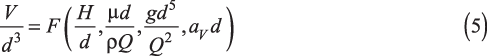
▲Figure 2. (a) The experimental liquid holdup, hL, in a packed bed is a function of the superficial velocity U of water (blue) and a more viscous water/glycerol mixture (orange). (b) The same data appear on a log-log plot against the dimensionless variable β = μUaV2/(ρg), overlaid with a power-law relationship having an exponent of 1/3 (green line) (7).
Figure 2a displays typical data from holdup experiments in which researchers used water (μ = 10–3 Pa-s) and a mixture of water and glycerol (μ = 10–2 Pa-s) over a packing with specific surface area aV = 203 m–1 to determine the holdup for a variety of superficial velocities, U (7). When the holdup is plotted against the dimensionless variable β in Figure 2b, it appears that data obtained with different liquids are indeed parts of the same function. This observation provides insight into the data because it suggests that the assumptions of homogeneous liquid distributions and of negligible effects of fluid inertia are met in the conditions of the figure. (This will be discussed later in more detail.) The dimensionless representation of Figure 2b provides a means to extrapolate the data to other liquids and packed beds, because the effects of all relevant variables, not only µ and U, are lumped into a single dimensionless number, β.
Guessing the shape of the unknown function
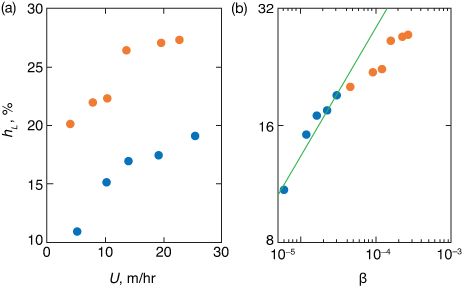
▲Figure 3. Fluid flow over a packed bed can be modeled as a liquid film flowing down a surface of inclination α at a flowrate per unit width, q.
To determine the mathematical form of the function F1, assume that the liquid flows as a thin film that covers the surface of the packing (Figure 3). The thickness of such a film is a classical problem in fluid mechanics (8), which can also be solved by dimensional analysis. The thickness, t (m), depends on the inclination, α (dimensionless), the flowrate per unit width of the surface, q (m2-s–1), the liquid’s viscosity, μ (kg-m–1-s–1), and density, ρ (kg-m–3), and gravity, g (m-s–2). Without an educated guess, these six variables would form a relationship among three dimensionless variables that provides little information.
Two educated guesses can be made. As discussed earlier, the flow is driven only by the component of gravity parallel to the slope, gsin(α), and inertia is negligible due to the laminar nature of the flow (as in Eq. 6). Thus, the three variables α, g, and ρ can appear only through their combination ρgsin(α). With four relevant variables — t, μ, q, and ρgsin(α) — and three dimensions, one dimensionless variable can be formed, namely t3ρgsin(α)/(μq).

Based on Eq. 2, this single dimensionless variable must be a constant, as there are no other relevant dimensionless variables for it to depend on. This produces the following expression for the thickness of the film:
where the constant dimensionless factor C1 is on the order of unity (i.e., between 0.1 and 10). Solving the Navier-Stokes equations yields C1 = 3.
Equation 8 can also be generated by applying a different method of dimensional analysis. That method, developed by Hellums and Churchill and described in the sidebar below, works when a mathematical model of the phenomenon with differential equations is available (9).
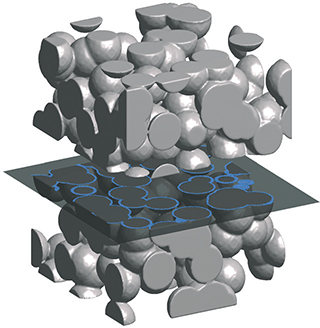
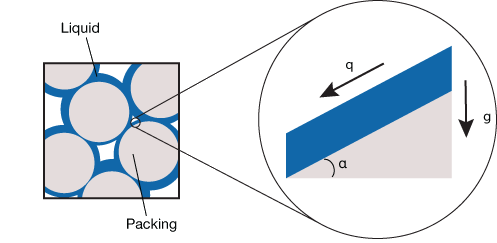
▲Figure 4. The intersection of the complicated 3D surface of the packing with a horizontal plane is a one-dimensional curve (blue). The length of the curve per unit area of the plane, L/S, is proportional to the specific area, aV , of the 3D surface, with a proportionality constant that depends on the packing.
The thickness and flowrate must now be related to the liquid holdup and the superficial velocity. The cross-section of the packing surface is a curve with a total length L (Figure 4). Because the liquid is limited to a thin film covering the surface and the total flowrate Q is equal to qL, the superficial velocity can be written as U = qL/S. The length of the curve per unit area, L/S, has the same dimensions as the specific surface area, aV, namely reciprocal length. Dimensional analysis then implies that L/S = C2aV , with a proportionality factor that varies from one packing to another.
The relationship between the flowrate, q, and the superficial velocity is therefore U = C2qaV. The thickness t is represented as the liquid volume per unit area of the packing, i.e., t = hL/aV. Combining these two geometric relationships with the expression for t in Eq. 8 yields:
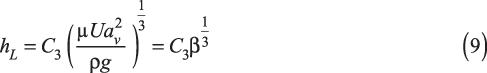
where sin(α) has been incorporated into the constant C3.

Equation 9 is compatible with the more general result given by Eq. 7, but it provides an explicit expression for the unknown function:

The constant dimensionless factor C3 can in principle be determined from one single experiment. This power law is in good agreement with the data in Figure 2, with C3 = 1.25, found from the intercept of the line on log-log scales. The empirical proportionality published by the manufacturer of the packing used for the data in Figure 2 has the form (10):
The values of the exponents of μ, U, and av in Eq. 9 are 1/3, 1/3, and 2/3, respectively. The agreement with Eq. 11 is striking considering that these exponents were obtained without solving any fluid mechanics equations. Moreover, the similarity between the theoretical and empirical exponents confirms the assumptions made in the dimensional analysis. In particular, it hints at a homogeneous distribution of the liquid throughout the packing.
Question the validity of guesses
In this approach to dimensional analysis, each educated guess reduces the number of variables needed to describe the system. It is through such systematic reduction that dimensional analysis is successfully applied to engineering problems. The comparison of collected data to calculated results reveals whether the assumptions are valid and the derived equations accurately describe the system.
In the trickle-bed reactor example, the thin-film assumption is valid as long as the thickness of the film, t, is significantly smaller than the characteristic size of the packing microstructure, 1/aV. Conversely, because aVt defines the liquid holdup, thin films are present when hL << 1. The downward deviation from the β1/3 trend in Figure 2b presumably reflects the breakdown of the thin-film assumption when the holdup reaches hL ≈ 0.2. Beyond that point, preferential paths are likely to form in the packing along which the liquid flows more easily than in the films.
Also in question is the general assumption of negligible inertial forces relative to viscous forces. This assumption justified discarding the density ρ from the variables, except from the product ρg, and the creation of Eq. 7, which states that hL depends on a single dimensionless variable β. Although this assumption is not restricted to thin-film configurations, thin films are assumed here to test the assumptions’ range of validity.
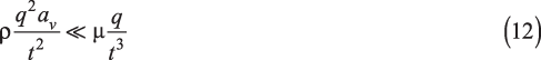
The order of magnitude of the local velocity of an infinitesimal liquid particle, u, in the packing is equal to q/t. The velocity of a given particle changes significantly over a distance on the order of 1/aV, so the inertial force per unit volume is on the order of ρu2aV = ρq2aV/t2. On the other hand, the viscous force on the same fluid element is proportional to μ times the second derivative of u with respect to a space coordinate. Because the derivative is the largest in the direction perpendicular to the film, the order of magnitude of the viscous force (per unit volume) is μu/t2 = μq/t3. The condition for negligible inertia can therefore be written as:

Using the relationships inferred between t, q, and U,Eq. 12 can be rewritten in terms of β:
With a surface area per unit volume of aV = 203 m–1, the condition is β < 3 × 10⁻⁵ for pure water and β < 9 × 10⁻⁴ for the water/glycerol mixture. Thus, Eq. 13 is reasonably satisfied for all the data points in Figure 2. Equation 13 defines the domain of validity of Eq. 7, and it is consequently also a necessary condition for Eq. 9 to hold true.
A useful technique
Dimensional analysis has many benefits for solving and simplifying practical engineering problems. It is a powerful tool to extrapolate data outside their measured range, optimize experimental and computational work, obtain first-order estimations, validate assumptions and identify their limits, and gain insight into a system at a very low cost. Its mathematical simplicity enables engineers to focus on the relevant phenomena without solving complex equations.
With dimensional analysis at hand, the complexity of a problem lies in the number of dimensional variables it contains. A dimensional analysis based on many more variables than fundamental units would be equivalent to solving a system with more unknown quantities than equations. An effective approach to dimensional analysis is to make assumptions to systematically reduce the number of variables, through either combining or discarding them. The malleability of this method based on educated guesses illuminates the strength of dimensional analysis to simplify a system by eliminating variables and experimental trials.
The Hellums-Churchill Method of Dimensional Analysis
When the problem at hand can be posed in the form of differential equations with boundary and/or initial conditions, the dimensional analysis technique developed by Hellums and Churchill can be used as an alternative to Buckingham’s Π theorem (9).
The Hellums-Churchill method has two main steps. First, for each dimensional variable X that appears in the equations, define an arbitrary reference variable X0 (dimensional), then define a dimensionless variable Y = X/X0. Express each equation and boundary condition in terms of Y. Second, replace each non-zero dimensionless group of variables with 1, then solve the resulting system of algebraic equations with unknowns X0. If the system is underdetermined, some X0 can be chosen arbitrarily to reduce the number of dimensionless parameters.
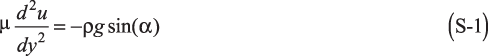
This general method is illustrated in the case of a viscous liquid flowing down a slope under the action of gravity (Figure 3). The flow is assumed to be one-dimensional, parallel to the substrate, steady, and invariant in the direction x along the substrate. The velocity field u(y) depends only on the distance y to the substrate. The Navier-Stokes equations are then reduced to:

for y ∈ [0,t ], with a no-slip boundary condition on the substrate (y = 0) and a stress-free boundary condition at the free surface (y = t), namely:
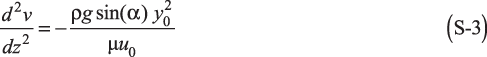
Next, introduce arbitrary length and velocity scales y0 and u0 and define z = y/y0 and v = u/u0. With these new dimensionless variables, the equations become:
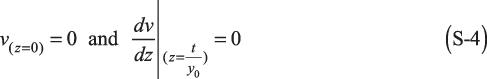
for z ∈ [0,t/y0 ], and
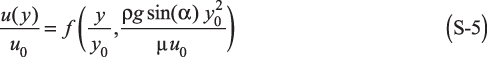
as boundary conditions. At this stage, although no equations have been solved, the solution is known to have the form:
where f is a yet-unknown function.

The only dimensionless group that appears in the problem is the one on the right-hand side of Eq. S-3, which is therefore one of the arguments of the unknown function f in Eq. S-5. The references y0 and u0 are arbitrary, and can be chosen so that the dimensionless group is equal to 1. The relationship becomes:

Moreover, the choice of y0 is still arbitrary, and it is convenient to choose y0 = t. With these particular choices, Eq. S-5 can be rewritten as:
The dimensionless group no longer appears in the arguments of the function f because it has been equated to one.

The flowrate per unit width of the slope, q, is calculated by integrating u(y) from y = 0 to t, namely:

This result is exactly Eq. 8 of the main text, where the unknown dimensionless proportionality factor here is expressed as the integral of f. Evaluating the numerical factor in Eq. 8 requires one to solve Eq. S-3, with the right-hand side set to 1, together with the boundary conditions in Eq. S-4. The solution is:
The integral in Eq. S-8 is therefore equal to 1/3, as noted in the main text. More complicated dimensionless problems would have to be solved numerically in order to determine the constant factor, but the scaling law itself can be obtained from dimensional analysis only.
To Explore Further
In addition to this analysis of liquid holdup in packed beds, this online version of this article includes supplementary material (see link below) that presents several classic engineering problems and shows how dimensional analysis with educated guessing can be used to solve them.
Acknowledgments
This work has been supported by the IAP 7/38 MicroMAST, which is funded by BELSPO (Belgian Science Office Policy). The authors are grateful to Professor D. Toye at the Univ. of Liège for stimulating discussions about the hydrodynamics of packed beds.
Nomenclature
| av | = surface area per unit volume of the packing |
| ai, bi, ci | = exponents in Buckingham Π functions |
| Ci | = dimensionless constant factor, on the order of unity |
| d | = diameter of the column |
| g | = standard acceleration due to gravity = 9.8 m/s2 |
| H | = height of the column |
| hL | = average holdup per unit volume |
| L | = curve length of packing cross-section |
| Q | = liquid flowrate |
| q | = flowrate per unit area width |
| S | = horizontal cross-sectional area of the packing |
| t | = thickness of the film |
| U | = superficial velocity |
| u | = order of magnitude of the local velocity of an infinitesimal liquid particle |
| V | = total volume of liquid in the packing |
| vi | = dimensional variable |
Greek Letters
| α | = angle of incline |
| β | = μUaV2/(ρg) = dimensionless variable used to study the liquid holdup |
| μ | = dynamic viscosity |
| Πi | = dimensionless group in Buckingham Π theorem |
| ρ | = density |
Literature Cited
- Alexander, R. M., “Walking and Running,” The Mathematical Gazette,80, pp. 262–266 (1996).
- Bohren, C. F., and A. B. Fraser, “Colors of the Sky,” Physics Teacher, 23, pp. 267–272 (1985).
- Sonin, A. A., “The Physical Basis of Dimensional Analysis,” 2nd Ed., MIT Dept. of Mechanical Engineering, http://web.mit.edu/2.25/www/pdf/DA_unified.pdf (2001).
- Barenblatt, G. I., “Scaling,” Cambridge University Press, New York, NY, pp. 2–11 (2003).
- Bird, R. B., et al., “Transport Phenomena,” 2nd Ed., Wiley, Hoboken, NJ (2007).
- Satterfield, C. N., “Trickle-Bed Reactors,” AIChE Journal, 21 (2), pp. 209–228 (1975).
- Aferka, S., et. al., “X-Ray CT Study of the Influence of Liquid Viscosity on Fluid Phase Distribution in Modular Catalytic Packings,” Chemical Engineering Transactions, 24, pp. 1429–1434 (2011).
- Landau, L. D., and E. M. Lifshitz, “Fluid Mechanics,” Butterworth-Heinemann, Oxford, U.K. (1959).
- Hellums, J. D., and S. W. Churchill, “Simplification of the Mathematical Description of Boundary and Initial Value Problems,’’ AIChE Journal,10 (1), pp. 110–114 (1964).
- Suess, P., and L. Spiegel, “Hold-Up of Mellapak Structured Packings,” Chemical Engineering and Processing, 31, pp. 119–124 (1992).
1

Copyright Permissions
Would you like to reuse content from CEP Magazine? It’s easy to request permission to reuse content. Simply click here to connect instantly to licensing services, where you can choose from a list of options regarding how you would like to reuse the desired content and complete the transaction.