Excelling with Excel #2 – Pivot Tables

Pivot tables are created from flat data

Tip#2: Pivot Tables

A tiny bit of theory first:

3-dimensional data structure created from a flat data table of 3 fields

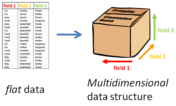
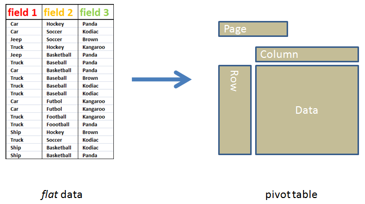
A pivot table does one thing: takes flat data and gives it depth. With this depth, we are able to sort and consolidate data in useful ways. A pivot table, in fact, can be thought of as a data structure of one or more dimensions. .. but "data structure" admittedly sounds scary. Instead, let's think about my favorite type of structure: a cardboard box.

Note: If this theory confuses you, don't worry! You do not need to understand this to use a pivot table. I mention this theory now because it may provide context for the more visual learners among us (yours truly) to better understand how pivot tables work.

What Does a Pivot Table Look Like?

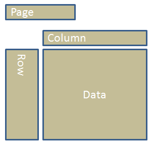
Pivot tables all follow the general layout below:

General format of a pivot table. There are 4 sections: Page, Row, Column, and Data

Now, observe where / how flat data is incorporated into this general pivot table layout:

The fields of flat data are placed into a pivot table

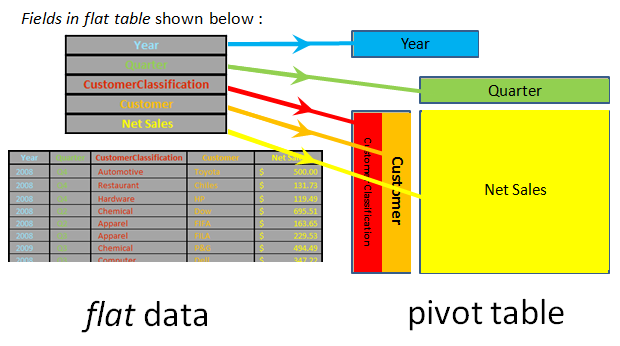
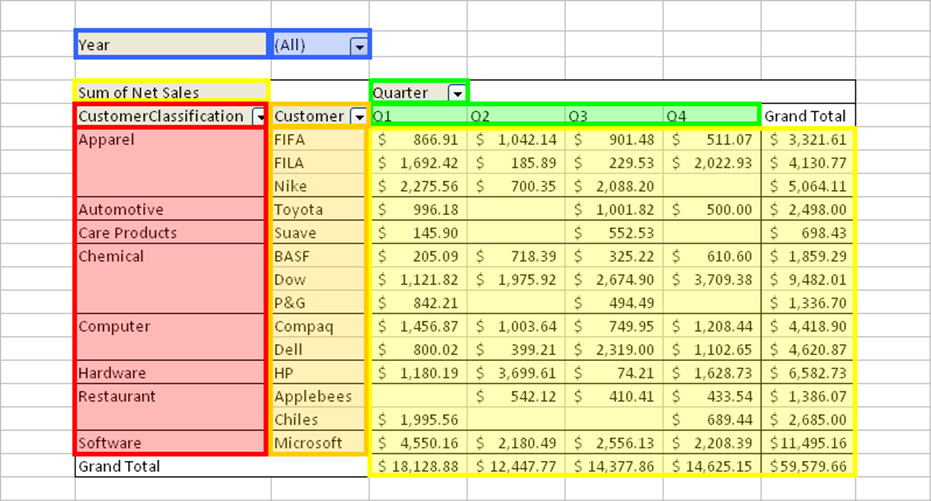
Below is the resulting pivot table after the incorporation of the fields shown above:

Pivot table after insertion of 5 fields noted above (with color formatting for clarity): Year, Quarter, Customer Classification, Customer, and Net Sales

How to Create a Pivot Table

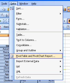
1) Data --> Pivot Table

2) Select "Microsoft Office list or database" and "Pivot Table". Click Next 3) Select your flat data (table of data). Click Next

4) Click Layout...

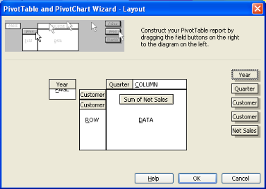
5) Choose the pivot table layout by dragging each field into a specific section of the pivot table. Click OK

6) Click Finish, and you're done (!!!)

k

Use: Creating Unique Lists

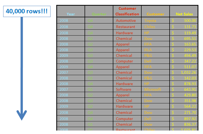
Let's say you have a HUGE sales transactions list (40,000 rows) with 5 different fields: Year, Quarter, Customer Classification, Customer, and Net Sales. From this, let's also assume you need to make a unique list of customers. Simple:

A HUGE 40,000 row data table (of sales transactions) that is just waitin' for a pivot table

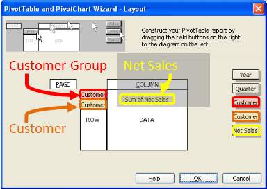
1) Data --> Pivot Table 2) Select "Microsoft Office list or database" and "Pivot Table". Click Next 3) Select your flat data (the aforementioned 40,000 row table of data). Click Next 4) Click Layout... 5) Choose the pivot table layout by dragging each field into a specific section of the pivot table. Click OK

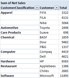
6) Click Finish, and you're done

Note: Each pivot table requires that you place at least one field into the Data section. In this case, I chose to put the Net Sales field in the Data section.

Note: You can remove all "Total" lines by right clicking any "Total" line and selecting "Hide".

Use: Consolidating Complex Data

Now, let's say you now need the cumulative Net Sales for each Customer, but these cumulative Net Sales figures need to be specific to Quarter (Q1, Q2 ,Q3 , or Q4) and Year (2007, 2008, or 2009). Just as simple:

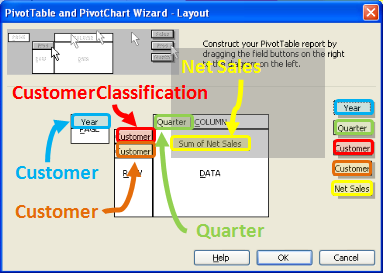
1) Data --> Pivot Table 2) Select "Microsoft Office list or database" and "Pivot Table". Click Next 3) Select your flat data (40,000 row table of data). Click Next 4) Click Layout... 5) Choose the pivot table layout by dragging each field into a specific section of the pivot table. Click OK 6) Click Finish, and you're done

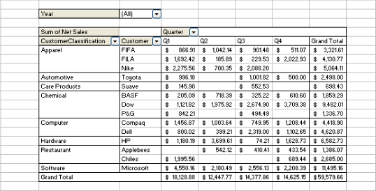
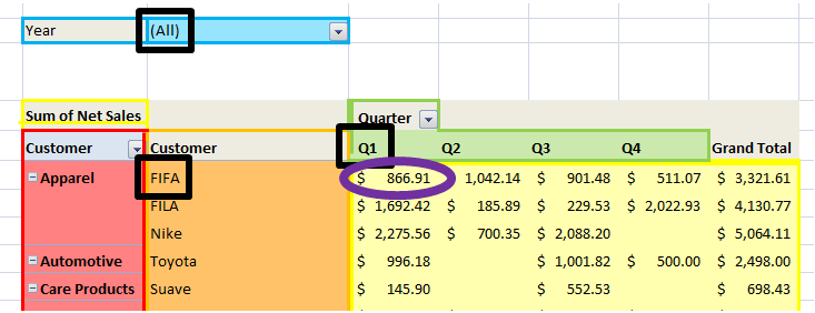
Let's take a look at this table above..

The pivot table above represents an immense amount of data manipulation (and a lot of time saved!). For instance, the FIFA Customer of the Apparel Customer Group has a cumulative Net Sales of $866.91 in all Q1 Quarters of all Years. If you didn't have a pivot table, acquiring this information would mean manually going through 40,000 rows of data!

Pivot table shown in the example above with the cumulative Net Sales for Customer FIFA in all Q1 Quarters

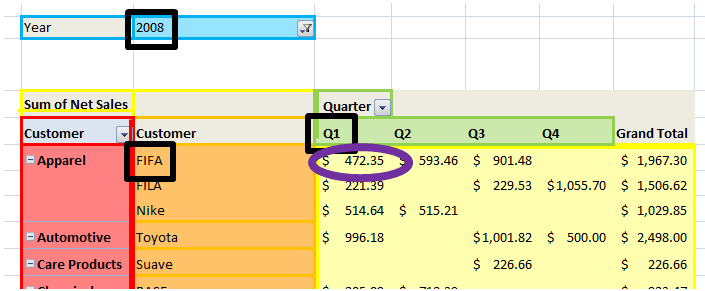
If we were to change the Year to 2008 instead of all, the cumulative Net Sales figure for the FIFA Customer (in the Apparel Customer Group) associated with Quarter Q1 would change to $472.35.

Pivot shown above with the cumulative Net Sales for FIFA in Q1 2008.

Summary

Anyone who deals with flat tables of data should know about pivot tables. They perform data manipulation (that may otherwise take hours) in a matter of seconds! And, best of all, they're simple to use: select desired data, drag'n'drop some fields, and you're done. Shake'n'bake.

If you have any questions about the content of this post, please leave a comment or contact my young professional ChE friend, Todd Krueger.

- Greg the Orange Cat