
Sections
Heat transfer to initiators, monomers, and other unstable materials can quickly become hazardous. This article proposes a simplistic model to analyze the temperature-time profile of an unstable chemical.
The chemical industry handles an increasing amount and variety of unstable chemicals. For example, many chemicals used to manufacture plastics, including peroxide-based initiators and olefinic monomers, are known to be unstable. The quantity of plastics produced worldwide has increased 12% over the five years from 2017 to 2021 and is expected to grow at a rate of at least 5% per year through 2030 (1, 2). Technological advancements are also expected to yield new products, including sustainable polymers, performance fibers used in textiles, biological-based medical-grade polymers, and more. Plastics manufacturers will see an increase in the variety and quantity of unstable chemicals due to limited and tailored formulations demanded by end customers. Therefore, the production and use of unstable initiators and monomers is also expected to increase, and manufacturers will need to develop a methodology for assessing and mitigating the increased risks associated with these chemicals.
Unstable chemicals typically generate heat at an accelerating rate as the storage and processing temperature increases. They can also release flammable and toxic gases that can create a greater risk of fires, explosions, and poisonings as they react or decompose. Therefore, chemical manufacturers and plant operators add chemical inhibitors and implement temperature control measures (i.e., refrigeration or vessel jacket quenching) to mitigate unwanted heating and runaway exothermic reactions. However, the inhibitor is consumed over time, and the rate of consumption increases exponentially with temperature. Typically, the inhibitor is also removed from the monomer before it is processed into a polymer. Temperature control may be impractical in certain situations, and manufacturers may be required to handle uninhibited monomers and initiators exposed to ambient or elevated temperatures.
The screening method presented in this article will help assess the risks associated with producing, handling, storing, and transporting unstable materials, in addition to identifying processes that require additional analysis. A heat transfer model and a chemical kinetics model are used in tandem to assess the performance of unstable chemicals. This article also discusses how to integrate potential hazards into a risk assessment methodology to predict thermal runaway. Given the many hazards associated with handling monomers and initiators, manufacturers can benefit from utilizing this screening approach to identify higher-risk chemicals and conditions that require further engineering controls.
Heat loss rate of packing
The heat transfer rate is driven by temperature difference and is proportional to the heat transfer coefficient. Although the temperature difference can change drastically over the course of a day (e.g., daytime and nighttime temperatures), the overall heat transfer coefficient, U, remains relatively constant over the area where the heat transfer occurs. The heat transfer rate, Q, can be expressed as:

where AS is the wetted surface area, and ΔT is the temperature difference. The thermal circuit analogy is used to calculate U:
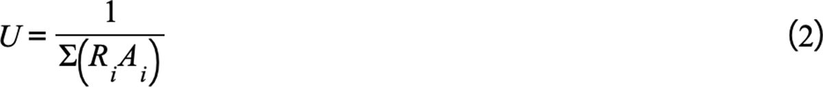
where Ri is the thermal resistance of an individual region of heat transfer (i.e., convection inside and outside the container) or layer of the container (i.e., conduction through the container wall and/or insulation layer) (3). Ai is the area over which the heat transfer occurs.
The product of U and AS can be determined experimentally by measuring the temperature change during the cooling of the vessel (4). To do so, it is recommended to use the “half-time of cooling” method by fitting the cooling data with a line generated by Eq. 3 (5).
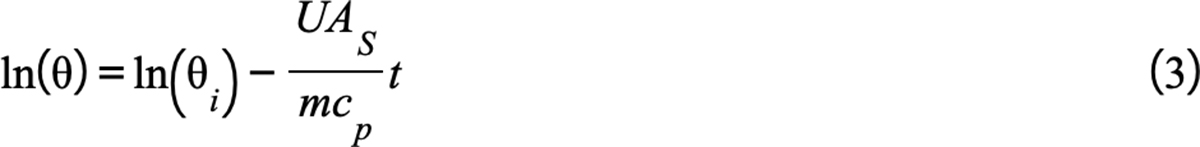
where θ is the temperature difference between the material and the environment at time t, θi is the temperature difference between the material and the environment at t = 0, m is the mass of the material, and cp is the specific heat of the material.
The Nusselt number, Nu, is a dimensionless number that compares the heat transfer by convection to that of conduction and is defined below:

where h is the convective heat transfer coefficient, L is the characteristic length of the object, and k is the thermal conductivity of the fluid. At an arbitrary fixed Nusselt number, a more thermally insulative fluid will exhibit lower convective heat transfer. Additionally, the thermal conductivity of a gas is typically at least an order of magnitude lower than the thermal conductivity of its liquid counterpart (3). Therefore, when storing liquids in containers, it is reasonable to assume that the heat transfer occurs through the wetted container surface only, and the heat transfer in the ullage (the amount by which a container falls short of being full) can be neglected.
One-gallon drum. Sheng et al. (4) measured the temperature change of a 1-gal drum of water as it cooled. A 17-cm dia. and 22-cm high drum was filled to about 90%, or 3.49 L, with water. The drum was heated in the oven at 76°C, then left to cool at ambient conditions. The cooling curve for water from data published by Sheng et al. is shown in Figure 1 (4).

▲Figure 1. This cooling curve of a 1-gal container filled with water to 90% of its volume helps numerically determine the overall heat transfer coefficient, U (4). The line’s slope is equal to –UAS/mcp, where m is mass, cp is specific heat, and AS is the wetted surface area. This line’s slope indicates that U equals 11.2 W/m2K.
Based on the linear fit of the data (Figure 1), the UAS value for the 1-gal container filled to 90% of its volume with water is equal to 1.182 W/K. When accounting only for the internal area wetted by water (AS = 0.105 m2), the U value is equal to 11.2 W/m2K, which is less than the value reported by Sheng et al. but consistent with previously published values (11.3 W/m2K) (4).
The relatively high ratio between the heat transfer rate and the thermal inertia in this configuration causes rapid heat transfer between the ambient environment and the contents. Therefore, the temperature of the contents readily approaches the ambient temperature. Heat generated by the contents of the package via exothermic polymerization or decomposition reactions is readily dissipated to the ambient environment, and the package is less likely to warm sufficiently to reach thermal runaway.
Figure 2 shows the cooling curve for methyl methacrylate (MMA) plotted from the data published by Sheng et al. (4). Based on a linear fit, the UAS value for the 1-gal container filled to 90% of its volume with MMA is 0.911 W/K. The overall heat transfer coefficient is 8.68 W/m2K. Although the overall heat transfer coefficient is lower than that reported by Sheng et al. (9.0 W/m2K), it is within the 10% experimental uncertainty reported in their publication (4).

▲Figure 2. Using the lumped capacitance model, this cooling curve of a 1-gal container filled with methyl methacrylate (MMA) to 90% of its volume indicates that the system’s overall heat transfer coefficient, U, is 8.68 W/m2K (4). The linear results and the R2 value being nearly equal to one indicate that the lumped capacitance model can be used to model the heat transfer between the ambient air and the MMA within this package.
A linear cooling curve is indicative of a package that can be modeled using the lumped capacitance method, which assumes that the temperature of the monomer/inhibitor within the package is completely uniform (i.e., a temperature gradient does not exist within the material). However, if a package does not exhibit a linear cooling curve, a temperature gradient may exist. A temperature gradient may also be observed when using multiple temperature probes during the cooling test. If the package exhibits a significant temperature gradient, the user is cautioned from using the lumped capacitance approximation, and more complex heat transfer models, such as computational fluid dynamics, may need to be incorporated into the screening method presented in this publication.
55-gal insulated drum. If experimental heat transfer data are not readily available like in the case of large or non-standardized containers, the product of the overall heat transfer coefficient and the heat transfer area, UAS, can be estimated from geometry and typical convective heat transfer coefficient values.
For a 55-gal insulated drum, the UAS can be estimated using the following equation:
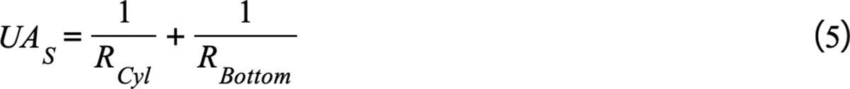
where RCyl is the resistance through the wetted shell of the drum and RBottom is the resistance through the wetted bottom of the drum. For more information on calculating RCyl and RBottom, see Ref. 5.
These calculations revealed that the UAS for a 55-gal insulated drum filled to 90% capacity is 1.387 W/K, given AS is 1.943 m2 and U is 0.714 W/m2K. In contrast to the 1-gal drum discussed above, the relatively low ratio of the heat transfer rate to thermal inertia in the 55-gal drum configuration leads to relatively slow heat transfer between the ambient environment and the contents. Therefore, the temperature of the contents approaches the ambient temperature much more slowly. Heat generated by the contents of the package is slowly dissipated to the ambient environment, and the package is more likely to warm up and reach thermal runaway.
Based on available data, a more accurate estimation of convective heat transfer coefficients can also be obtained by employing the appropriate Nusselt number correlations on a case-by-case basis. If temperature gradients are known to exist within the package, the user is cautioned from using the lumped capacitance method, and more complex heat transfer models may need to be incorporated into the screening method presented in this publication.
Kinetic properties of unstable chemicals
To properly classify unstable materials for shipment, it is necessary to determine the heat transfer properties of the packaging used to transport them. For example, the United Nations Recommendations on the Transport of Dangerous Goods (UNRTDG) Manual of Tests and Criteria (6) considers self-heating solids and monomers to be Class 4, Div. 4.1 substances if their self-accelerating decomposition temperature (SADT) or self-accelerating polymerization temperature (SAPT) is 75°C (167°F) or less within the packaging used, the heat of reaction is greater than 300 J/g, and they do not meet other criteria specified in Classes 1–8. Further, the substances must be temperature controlled if the SADT or SAPT is less than 50°C (113°F) within intermediate bulk containers (IBC) or packaging, and less than 45°C (131°F) within a portable tank. These criteria can also be incorporated into a kinetic model to assess risks associated with the manufacture, storage, and handling of unstable materials.
Calculation of the self-heating rate from accelerating rate calorimetry data. Tert-butyl peroxybenzoate (TBPB) and MMA are both commonly used and transported hazardous materials. TBPB decomposes and MMA autopolymerizes at increasing rates as they heat up, and both reactions generate heat. Although these reactions occur at near-negligible rates at low temperatures, if the heat from these reactions is not effectively dissipated to the ambient environment (e.g., when stored in insulated packaging), the products will warm up over time and eventually reach thermal runaway, and the temperature rise becomes almost instantaneous. Heat, decomposition products, and vapors generated from a runaway reaction can damage equipment, potentially exposing personnel to toxic, hot, and flammable vapors. If the temperature of the vapors is above their autoignition temperature or if there is a credible ignition source, a flash fire or explosion with damaging overpressure can occur, exposing personnel to additional hazards.
In order to assess the conditions that result in these catastrophic scenarios, accelerating rate calorimetry (ARC) data were extracted for liquid TBPB and liquid MMA with 25 ppm mono-methyl ether of hydroquinone (MEHQ) inhibitor to determine the relationship between temperature rise (dT/dt) and temperature and assess chemical instability (4, 7). A zeroth-order Semenov model, which is applicable to low-viscosity self-reactive monomer or organic peroxide systems, was assumed to apply (4, 7, 8). For reaction kinetics to be considered zeroth order, the natural log of dT/dt vs. inverse temperature must be linear. Although MMA will transition to a high-viscosity system as it self-polymerizes, which can create a large temperature gradient within the liquid, the Semenov model is applicable to the initial rate of reaction (i.e., at low conversion, <20%) (4). MMA does not polymerize and generate heat until after the inhibitor has been consumed. Therefore, the exotherm detected by ARC occurs after the inhibitor has been consumed, and the kinetic parameters derived from the ARC data for MMA are applicable to uninhibited MMA. For inhibited MMA and other inhibited monomers, additional consideration must be given to the time required to consume the inhibitor prior to the start of self-heating (possibly on the order of weeks or longer at ambient temperatures), which is outside the scope of this publication.
Although zeroth-order reaction kinetics are a conservative approximation for reactions that follow nth-order Arrhenius kinetics, many systems follow more complex reaction mechanisms, including autocatalytic and multistage reaction systems. Therefore, the method presented herein should be considered a screening tool, and more complex reaction mechanisms should be applied to systems known to significantly deviate from nth-order Arrhenius-type reaction rates.
The rate change in concentration (dC/dt) is a function of concentration, C, the rate constant as a function of temperature, k(T), and the order of reaction, n (8). The rate constant, k(T), is expressed by the Arrhenius equation, shown below.

where A is the pre-exponential factor, R is the ideal gas constant, and EA is the activation energy (9).
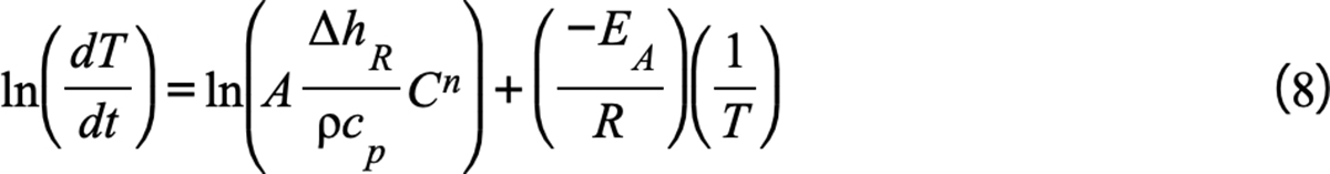
Substituting the rate constant for the Arrhenius equation, dT/dt can be written using the following equation:
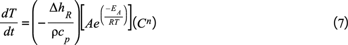
Here, ρ is density and ΔhR is the heat of reaction. The natural log of Eq. 7 results in the following equation:
Given that the ARC data were collected while the reactants were being consumed, plotting Eq. 8 will yield a linear relationship if the reaction rate is zeroth order (n = 0) (Figure 3). The values of dT/dt shown in Figure 3 have been corrected to account for the heat absorbed by the ARC vessel using the Fisher method presented by Kossoy et al. (10).

▲Figure 3. This linear regression of ln(dT/dt) vs. inverse temperature for MMA with 25 ppm mono-methyl ether of hydroquinone (MEHQ) inhibitor and tert-butyl peroxybenzoate (TBPB) helps determine the activation energy, EA, of each species. Given that the slope of each line is equal to –EA/R (where R is the ideal gas constant), the EA for MMA is 71,165 J/mol and the EA for TBPB is 139,509 J/mol.
The R2 values of the linear regression in Figure 3 are essentially uniform, and therefore, reaction kinetics for MMA and TBPB can be approximated by a zeroth-order reaction rate during the initial stages of the reaction. Per Eq. 8, the slope of the regression, mG, is given by –EA/R with units of K and the intercept, bG, is given by ln(AΔhR/[ρcp]) with units of ln(K/sec) since Cn = 1 for zeroth-order reactions. The activation energy, EA, calculated from the slope is 71,165 J/mol for MMA and 139,509 J/mol for TBPB.
Calculation of time to maximum rate
Time to maximum rate (TMR) represents the amount of time, given an initial temperature, necessary to reach the maximum decomposition rate under adiabatic conditions (i.e., all heat generated by the material is absorbed by the material, and no heat is lost to the environment). Therefore, this parameter can be used to evaluate the minimum time necessary for exothermic decomposition given an initial starting temperature (11).
The starting temperature that corresponds to a 24-hr TMR (TMR24) — the starting temperature at which it takes 24 hours to reach maximum rate — is used as a reference value for comparing data on thermal stability, as it aligns with standard operation cycles in many industries, enabling them to transport, monitor, and plan reactions of certain chemicals over a complete day. If a reaction is likely to reach a maximum rate within 24 hours at an ambient temperature (e.g., TMR24 = 25°C), this indicates a need for immediate intervention or additional safety measures.
Townsend and Tou (12) developed equations for the self-heating rate, TMR, and temperature of no return (TNR) based on ARC data. Wilberforce (13) and Whitmore (14) expanded on this methodology and proposed a TMR curve developed with ARC data to calculate the SADT. Their method of determining TNR and SADT has been widely used and accepted (15, 16). For reactions with high activation energy (>83,680 J/mol) (12), TMR can be expressed as the following equation:
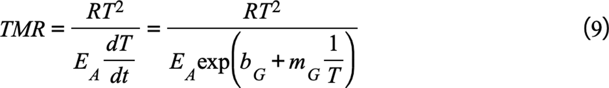
where T is the temperature of the material, bG is the intercept and mG is the slope of the line in Figure 3 calculated from Eq. 8, and EA is the activation energy calculated from mG. The simplified form of the TMR equation shown in Eq. 9 is acceptable for reactions with activation energies slightly below 83,680 J/mol (e.g., MMA) for starting temperatures where TMR >1 hr, since the neglected term is on the order of a few minutes.
Parameters used to calculate the TMR for MMA and TBPB extracted from previously published work and publicly available thermodynamic data are summarized in Table 1 (4, 7, 17). Zeroth-order reaction kinetics (i.e., n = 0) were assumed (18). The TMR24 is extrapolated from the TMR vs. temperature plot shown in Figure 4 (19). MMA and TBPB have TMR24 values of 44.4°C and 57.7°C, respectively.
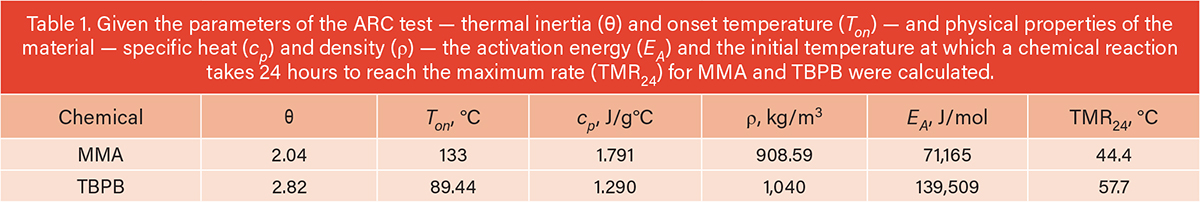
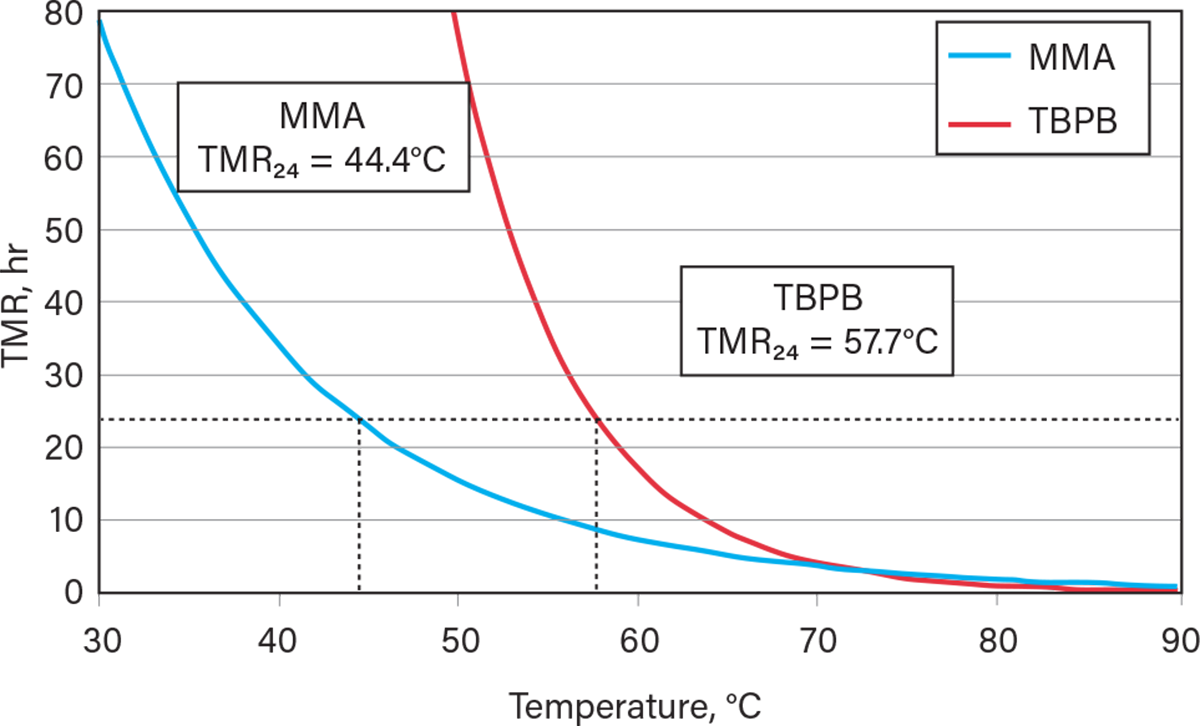
▲Figure 4. This graph displays the time to maximum rate (TMR) for MMA and TBPB. The initial temperature at which the system reaches the maximum rate of reaction in 24 hours (TMR24) is used as a reference value for comparing data on thermal stability. This time scale aligns with standard operation cycles in many industries.
Figure 4 demonstrates that neither chemical will readily exhibit runaway exothermic conditions at typical ambient temperatures, that is, below 25°C. However, additional precautions are warranted in hot weather, such as tropical climates or regions with high solar insolation. For example, the Methacrylate Producers Association recommends storing MMA below 40°C (104°F) and acknowledges that temperatures exceeding 45°C (113°F) indicate an ongoing polymerization reaction. This is consistent with the temperature at which it takes uninhibited MMA to fully runaway within 24 hr as calculated by the method presented in this paper (20). Zhou et al. experimentally determined that TBPB has a TMR24 of 55.61°C, consistent with the TMR24 value calculated by the method presented in this paper (21).
Calculation of SADT or SAPT
To calculate the SADT or SAPT using the Semenov model, the heat loss curve (QL), which is a linear line with the slope of the heat loss rate, is drawn tangential to the heat generation curve (QG) developed from the ARC data (Figure 5). The heat loss curve is dependent on the sample mass (ρV), overall heat transfer coefficient (U), and wetted surface area (AS) of the packaging, given by the following equation:
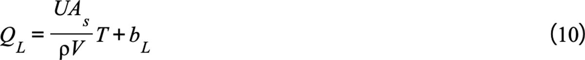
where bL is the intercept of the heat loss curve when drawn tangential to the heat generation curve.
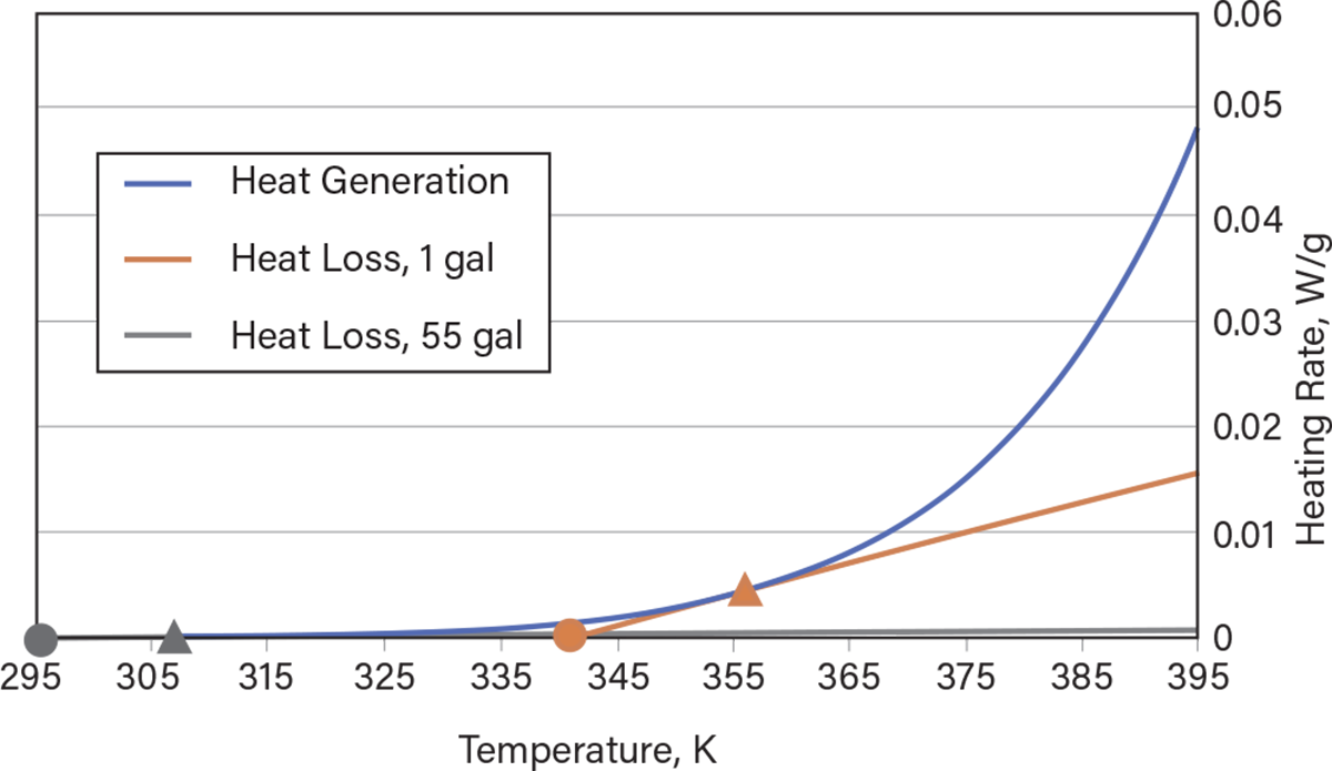
▲Figure 5. This accelerating rate calorimetry (ARC) data, corrected using the Fisher method, helps determine the temperature of no return, TNR, and critical temperature, TCR, of MMA packaged in a UN 1A1 1-gal drum and UN 1A2 55-gal drum. The TNR is determined by where the heat loss curve is tangential to the heat generation curve (triangles). The TCR is then determined from where the heat loss curve is zero, i.e., x-axis intercepts (circles).
The heat generation curve, QG, is calculated by multiplying the temperature rate of change (Eq. 7) with the specific heat. QG can be represented using the following equation:

The TNR is the temperature at which the QG curve has the same slope as the QL curve. Above the TNR, heat generation exceeds the maximum rate of cooling, and the system cannot be prevented from undergoing thermal runaway. The slope of the heat generation curve is determined by taking the derivative of Eq. 11 with respect to temperature (4).
The critical temperature (TCR) is determined from the heat loss curve’s x-axis intercept (Figure 5). The intercept of the heat loss curve (bL) is determined by setting Eq. 10 equal to Eq. 11 and setting the temperature equal to TNR.
The SADT or SAPT is determined by rounding TCR up to the next higher multiple of 5°C (4). Figure 5 demonstrates the process of calculating TNR and TCR from the heat generation curve for MMA and the heat loss curves for 1-gal and 55-gal packages. SAPT for MMA in a 1-gal drum reported here is consistent with values reported by Sheng et al. (4). The process for calculating these parameters for TBPB is shown in Figure 6.
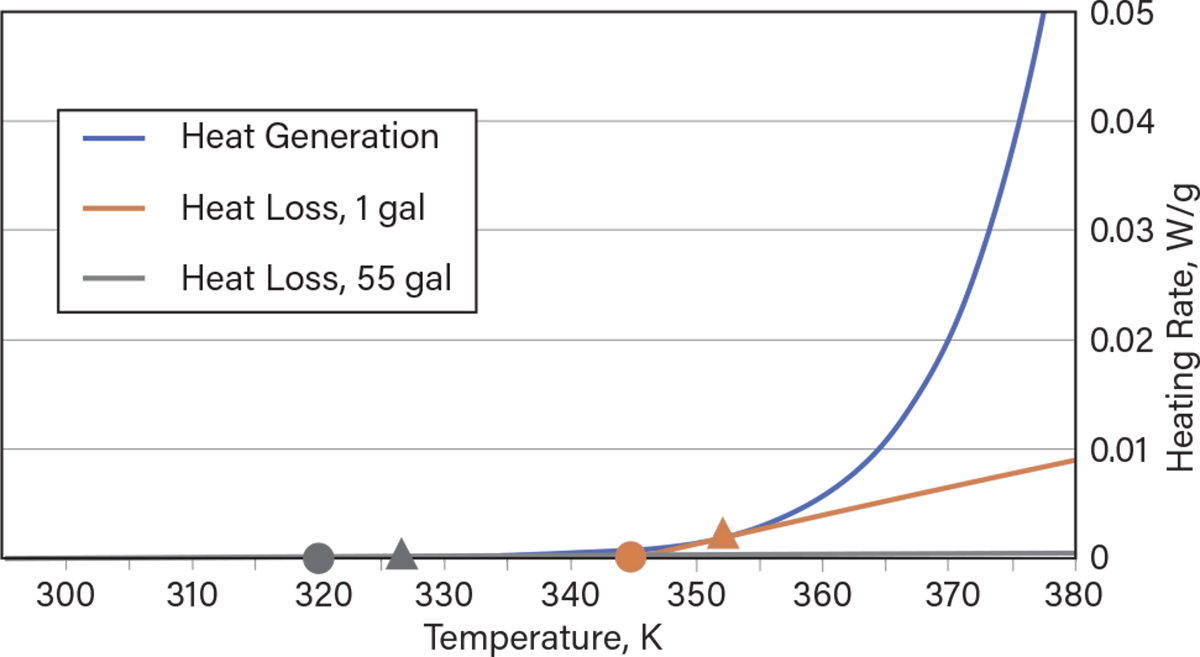
▲Figure 6. Using the same process as Figure 5, this ARC data helps determine the TNR (triangles) and TCR (circles) of MMA packaged in a 1-gal drum and 55-gal drum.
Since the heat loss rate is proportional to the overall heat transfer coefficient (U) and the ratio of the wetted surface area of the package to the volume of the material (A/V), decreasing U (e.g., by adding insulation) and/or decreasing A/V (e.g., by increasing sample size) decreases the SADT.
Heat transfer model
Once the adiabatic behavior (e.g., change rate of temperature with respect to time and TMR24) of an unstable material is determined, a heat transfer model can be applied to understand how it will respond to heat gained or lost to the environment.
Lower heat transfer rates (e.g., within insulated containers) will cause the material to slowly heat up when exposed to warmer ambient temperatures, which might allow longer storage times. However, if the material also generates significant heat from an exothermic reaction, heat loss to the environment is also slower. This implies that, once the material self-heats above ambient conditions, it will more readily achieve runaway conditions. For high heat transfer rates (e.g., uninsulated containers), the opposite is true. Chemical handlers must understand these trade-offs to select appropriate container and storage conditions.
Heat transfer between stored chemicals and the environment occurs continuously and is based on their temperature difference. Heat conduction through the container as well as heat convection at the container walls must be considered. Factors including heat generation within the container due to decomposition or side reactions as well as agitation are also relevant.
The total temperature change of the container can be expressed as the sum of the individual contributions, including the temperature change due to the heat transfer with the environment (ΔTHT), heat generated by equipment (e.g., agitation) (ΔTAG), any decomposition/polymerization reactions (ΔTCR), and parasitic/side reactions (ΔTother). For more information on calculating these values, see Ref. 5.
Heat transfer with the environment. Temporal temperature change can often be modeled via a lumped capacitance model (3), which assumes uniform temperature within an object. Assuming negligible temperature gradients is appropriate for objects with high thermal conductivity, small mass, or agitated containers.
In the case of liquid in a container, the lumped capacitance model can be used for relatively small masses and for agitated liquids where the temperature is relatively uniform throughout. However, the convective heat transfer inside and outside of the container and heat conduction through container walls must be considered.
Heat generated from equipment. While equipment such as agitators and circulators are often used in chemical processes, they can introduce unintended heat to the process. These sources are often neglected during process design and may cause thermal-runaway incidents (22). During startup, heat dissipation from the equipment might be reduced because part of the energy is used to reach steady-state operating conditions. The change in temperature due to heat generated by equipment (ΔTAG) is shown in Eq. 12:
where Ẇ is the energy contributed by the machinery.
Heat generated from decomposition reactions. For a decomposition or polymerization reaction that can be approximated as a zeroth-order reaction, the Arrhenius-type linearization expressed in Eq. 8 can be used to determine heat generation and the associated temperature change.
Heat generated from unintended side reactions (contamination). In some instances, the presence of contaminants can also generate heat if they cause parasitic or side exothermic reactions. A simplified case of heating due to a side reaction, ΔTother, with a constant heat generation rate, ṙ, can be calculated using the following equation:
Risk assessment application. Consider a condition where MMA is stored in a 55-gal insulated tank. The MMA was removed from refrigeration at 10°C and exposed to an ambient temperature of 20°C, which is below the SADT. Due to the effects of heat transfer and heat generated from the self-polymerization reaction, the temperature of the MMA will increase until the heat generated from the polymerization reaction is equal to the heat lost to the environment. The temperature approaches an asymptote of 25.6°C, which is between the TCR (22.0°C) and TNR (33.0°C), and therefore, the MMA is not expected to run away under these conditions (Figure 7).

▲Figure 7. The temperature profile of MMA in a 55-gal insulated drum exposed to an ambient temperature of 20°C without agitation, with agitation, and with agitation that is turned off when the temperature of the MMA reaches the TNR. This simulation demonstrates how heat from mechanical agitation, a heat source that is frequently overlooked during the design process, can be sufficient to heat a batch of MMA above the TNR if safety mechanisms are not implemented.
Now consider the same condition, but the MMA is also exposed to mechanical agitation from a stirrer that imparts 20 W of frictional heat generation (Figure 7). The additional heat causes the MMA to undergo a self-accelerating polymerization reaction. However, if the stirrer is programmed to turn off after the temperature of the MMA reaches the TNR (Figure 7), the MMA cools to the same temperature as the unagitated MMA.
As part of the risk assessment, it may be determined that the agitator should be turned off when the MMA reaches a temperature that is 5°C below the TNR to incorporate a margin of safety. Other process-specific scenarios should also be considered during a risk assessment, for example, evaluating whether refrigeration would be effective at preventing a runaway reaction and determining effective temperatures of the heat transfer medium within the storage tank jacket. Acceptable storage times might also be evaluated based on the analysis presented to ensure stored chemicals do not undergo unintended runaway reactions.
Closing thoughts
This article reviewed historical case studies where unstable materials underwent a self-accelerating decomposition or polymerization reaction. Additional study of unstable materials is necessary because the number of incidents has continued to increase over the past two decades.
The screening method presented in this paper can help assess which chemicals and processes warrant further evaluation. Such evaluation may include replacing the lumped capacitance heat transfer model with a more robust heat transfer model, including one-dimensional, two-dimensional, or computational fluid dynamics models. Additionally, the zeroth-order kinetics model can be replaced with more robust kinetics models, including those for autocatalytic or multistage reaction systems. In certain situations, modeling may need to be supplemented with full-scale recreations and experiments.
*This article is a condensed version of a paper published in Process Safety Progress, “Considerations for the safe handling and processing of unstable materials,” doi: 10.1002/prs.12652 (Oct. 11, 2024).
Nomenclature
| A | = pre-exponential factor, mol/sec (for first-order reactions) |
| Ai | = area over which heat transfer occurs |
| AS | = wetted surface area, m2 |
| bG | = intercept on a first-order reaction linearization like Figure 3 |
| bL | = the intercept of the heat loss curve when drawn tangential to the heat generation curve |
| C | = concentration, mol/L |
| cp | = specific heat of the material, J/g-K |
| dC/dt | = rate of change in concentration, m/sec-L |
| dT/dt | = rate of change in temperature, K/sec or K/min |
| EA | = activation energy, J/mol |
| h | = convective heat transfer coefficient, W/m2K |
| k | = thermal conductivity, W/m-K |
| k(T) | = rate constant, mol/sec (for first-order reactions) |
| L | = characteristic length, m |
| m | = mass of the material, g |
| mG | = slope on a first-order reaction linearization like Figure 3 |
| Nu | = Nusselt number |
| n | = order of reaction |
| Q | = heat transfer rate, W |
| QL | = heat loss |
| R | = ideal gas constant, J/mol-K |
| RBottom | = resistance through the wetted bottom of the drum, Ω |
| RCyl | = resistance through the wetted shell of the drum, Ω |
| Ri | = thermal resistance of an individual region of heat transfer, Ω |
| ṙ | = heat generation rate, W/g |
| t | = time, sec, min, hr |
| U | = overall heat transfer coefficient, W/m2K |
| Ẇ | = energy generated by the machinery, W |
| Greek Letters | |
| ΔhR | = heat of reaction, J/mol |
| ΔT | = temperature difference, K |
| ΔTAG | = heat generated by machinery, K |
| ΔTother | = heat generated from parasitic/side reactions, K |
| θ | = temperature difference between the material and the environment at time t, K |
| θi | = temperature difference between the material and the environment at t = 0, K |
| ρ | = density, kg/m3 |
Literature Cited
- Statista Research Department, “Annual Production of Plastics Worldwide from 1950 to 2022,” Statista, https://www.statista.com/statistics/282732/global-production-of-plastics-since-1950 (Nov. 21, 2024).
- SkyQuest, “Polymer Market Size, Share, Growth Analysis, By Type (Polypropylene, Polyethylene), By Process, By End Use, By Region — Industry Forecast 2025-2032,” https://www.skyquestt.com/report/polymer-market (Dec. 2024).
- Bergman, T. L., et al., “Fundamentals of Heat and Mass Transfer,” 8th ed. John Wiley & Sons, Hoboken, NJ (Dec. 2018).
- Sheng, M., et al., “Calorimetric Method to Determine Self-Accelerating Polymerization Temperature (SAPT) for Monomer Transportation Regulation: A Heat Balance Approach,” Organic Process Research & Development, 23 (5), pp. 750–761 (Apr. 18, 2019).
- Ott, B., et al., “Considerations for the Safe Handling and Processing of Unstable Materials,” Process Safety Progress, pp. 1–9 (Oct. 11, 2024).
- United Nations, “Manual Tests and Criteria,” 7th ed., U.N., https://unece.org/fileadmin/DAM/trans/danger/publi/manual/Rev7/Manual_Rev7_E.pdf (2019).
- Gong, L., “Thermal Hazards and Initial Decomposition Mechanisms Study of Four Tert-Butyl Organic Peroxides Combining Experiments with Density Functional Theory Method,” Thermochimica Acta, 708 (Feb. 2022).
- Kossoy, A. A., and I. Y. Sheinman, “Comparative Analysis of the Methods for SADT Determination,” Journal of Hazardous Materials, 142 (3), pp. 626–638 (Apr. 11, 2007).
- Vyazovkin, S., “Isoconversional Kinetics of Thermally Stimulated Processes,” Springer, Princeton, NJ (Mar. 20, 2015).
- Kossoy, A. A., et al., “Mathematical Methods for Application of Experimental Adiabatic Data – An Update and Extension,” Journal of Loss Prevention in the Process Industries, 33, pp. 88–100 (Jan. 2015).
- Keller, A., et al., “Estimation of the Time to Maximum Rate Using Dynamic DSC Experiments,” Journal of Loss Prevention in the Process Industries, 10 (1), pp. 31–41 (Jan. 1997).
- Townsend, D. I., and J. C. Tou, “Thermal Hazard Evaluation by an Accelerating Rate Calorimeter,” Thermochimica Acta, 37 (1), pp. 1–30 (Apr. 1, 1980).
- Wilberforce, J. K., “The Use of the Accelerating Rate Calorimeter to Determine the SADT of Organic Peroxides,” Columbia Scientific Industries Corp. (July 1981).
- Whitmore, M. W., and J. K. Wilberforce, “Use of the Accelerating Rate Calorimeter and the Thermal Activity Monitor to Estimate Stability Temperature,” Journal of Loss Prevention in the Process Industries, 6 (2), pp. 95–101 (Mar. 1993).
- Yao, H., et al., Investigation of Pyrolysis Kinetics, Mechanism and Thermal Stability of Tert-Butyl Peroxy-2-Ethyl Hexanoate,” Process Safety and Environmental Protection, 160, pp. 734–748 (Apr. 2022).
- Fisher, H. G., and D. Goetz, “Determination of Self-Accelerating Decomposition Temperature Using the Accelerating Rate Calorimeter,” Journal of Loss Prevention in the Process Industries, 4 (5), pp. 305–316 (Oct. 1991).
- Green, W., and R. West, “RMG—Reaction Mechanisms Generator,” Massachusetts Institute of Technology, https://rmg.mit.edu (June 18, 2024).
- Sun, J., et al., “A Study of Self-Accelerating Decomposition Temperature (SADT) Using Reaction Calorimetry,” Journal of Loss Prevention in the Process Industries, 14 (5), pp. 331–336 (Sept. 2001).
- UN Sub-Committee of Experts on the Transport of Dangerous Goods, “Proposal to Amend the Proper Shipping Name of Crotonaldehyde (UN 1143) / Transmitted by the International Council of Chemical Associations,” U.N., https://digitallibrary.un.org/record/521371?ln=en&v=pdf (April 2004).
- Methacrylate Producers Association, “Methacrylate Esters Safe Handling Manual,” Methacrylates Sector Group of the European Chemical Industry Council, https://www.petrochemistry.eu/wp-content/uploads/2019/08/Methacrylate-Esters-Safe-Handling-Manual-Rev-FINAL-8-22-19.pdf (2019).
- Zhou, H. L., et al., “Thermal Hazard Assessment of Tert-Butyl Perbenzoate Using Advanced Calorimetric Techniques and Thermokinetic Methods,” Journal of Loss Prevention in the Process Industries, 85 (Oct. 2023).
- Barton, J. A., and P. F. Nolan, “Incidents in the Chemical Industry Due to Thermal-Runaway Chemical Reactions,” IChemE Symposium Series No. 115 (1989).

Copyright Permissions
Would you like to reuse content from CEP Magazine? It’s easy to request permission to reuse content. Simply click here to connect instantly to licensing services, where you can choose from a list of options regarding how you would like to reuse the desired content and complete the transaction.